Methodology
Test sequence set
The video sequences stated below are used in educational purpose only. All samples are taken from openly available sources and open video sets with respect to the creators.
The following sequence set is defined to perform testing:
| Scene type | Source |
|---|---|
| Action | Tears of Steal |
| Animation | Netflix Sol Levante |
| Film | Harmonic Venice Carnival Netflix Food Market Netflix Meridian Netflix Wind and Nature |
| Nature | Harmonic Birds of Pray Harmonic Monkey Pool Harmonic Monkey Fur Closeup Harmonic Waterfall |
| Static scene | ProArtInc Ruby Beach campfire |
| Teleconference | MixKit Coworkers |
Video samples:
All input video sequences are to be encoded to the respected bitrates depending on frame size
| Frame size | Bitrates |
|---|---|
| 256×144 | “27K”, “62K”, “97K”, “132K”, “167K”, “203K”, “238K”, “273K”, “308K”, “343K” |
| 412×232 | “49K”, “111K”, “174K”, “236K”, “299K”, “361K”, “424K”, “486K”, “549K”, “611K” |
| 640×360 | “95K”, “216K”, “338K”, “459K”, “581K”, “702K”, “824K”, “945K”, “1067K”, “1188K” |
| 852×480 | “148K”, “337K”, “526K”, “714K”, “903K”, “1092K”, “1281K”, “1469K”, “1658K”, “1847K” |
| 1280×720 | “260K”, “591K”, “921K”, “1252K”, “1583K”, “1913K”, “2244K”, “2575K”, “2905K”, “3236K” |
| 1920×1080 | “461K”, “1046K”, “1632K”, “2217K”, “2802K”, “3388K”, “3973K”, “4558K”, “5144K”, “5729K” |
| 2560×1440 | “671K”, “1523K”, “2374K”, “3226K”, “4078K”, “4929K”, “5781K”, “6633K”, “7484K”, “8336K” |
| 3840×2160 | “1000K”, “2333K”, “3667K”, “5000K”, “6333K”, “7667K”, “9000K”, “10333K”, “11667K”, “13000K” |
Quality metrics
PSNR: https://en.wikipedia.org/wiki/Peak_signal-to-noise_ratio
SSIM: https://en.wikipedia.org/wiki/Structural_similarity_index_measure
VMAF: https://github.com/Netflix/vmaf
Bitrate range codec comparison
Codec comparison for the bitrate range uses the method of Gisle Bjontegaard: https://www.itu.int/wftp3/av-arch/video-site/0104_Aus/VCEG-M33.doc.
The following channels are use for different metrics
| Metric | Channel |
|---|---|
| VMAF | All |
| PSNR | All |
| SSIM | Y |
What is BDBR?
If you have ever engaged in video coding quality analysis and compared different codecs, you have likely used rate-distortion or RD curves.
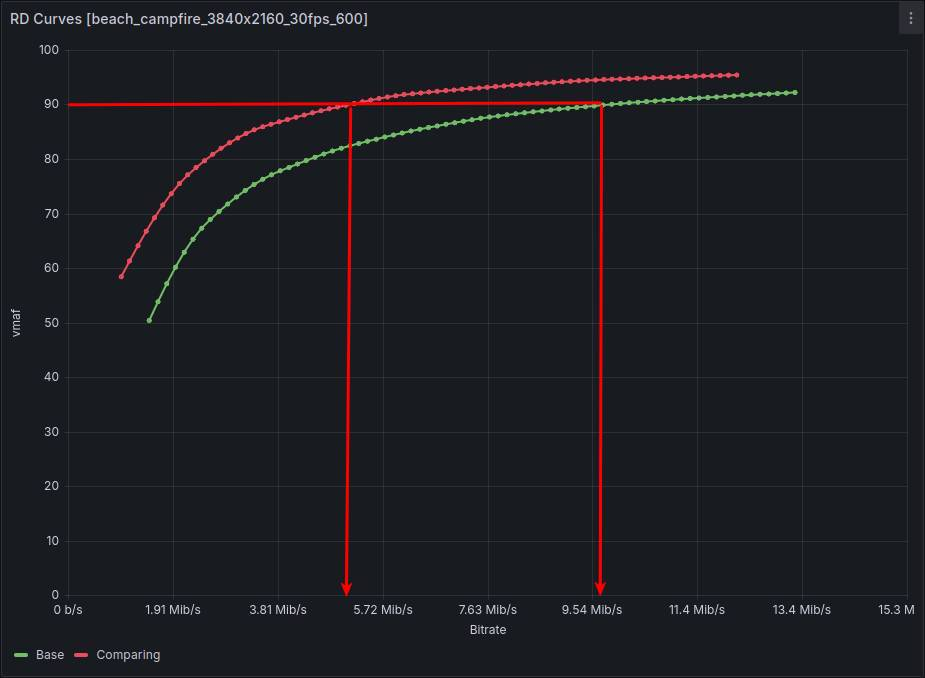
Since the X-axis represents bitrate values and the Y-axis represents a quality metric, a higher curve indicates the codec encodes with higher quality at the same bitrate. Visually, the curves are quite close to each other, and one might erroneously conclude that their quality difference is not significant. However, BDBR indicates the codec with the green curve needs to add, on average, 45% more bitrate to achieve the quality of the second one.
When asking the question, “how much more or less bitrate is needed to achieve the quality of the compared codec?”, one needs to draw a horizontal line at a given quality level and observe at which bitrate points it intersects the curves. For this purpose, an “inverted” graph is more suitable, where the X-axis represents quality and the Y-axis represents the required bitrate:
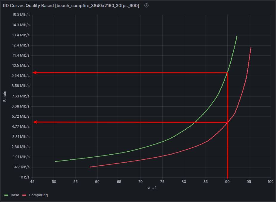
Now the graph visually aligns with the question. A “higher” curve now indicates the codec lacks sufficient bitrate to match the quality of the second one.
Alright, we have determined that at the point of 90 VMAF, the “red” codec requires 5.15 Mbps, while the green one requires 9.89 Mbps. But this is not enough to understand how much better one codec is than the other. One could calculate the difference at the boundaries and average the values, continuing to add points to average the overall indicator ad infinitum. This essentially boils down to the ratio of the areas under the curves.
To obtain the ratio of the areas under the curves, one must compute the polynomials describing the quality-to-bitrate dependency, determine the boundaries of bitrate intersection for the two codecs, and integrate the function over this interval.
This is precisely what Gisle Bjontegaard proposed in 2001 for comparing codec quality. Technically, 4 points are sufficient for this approach. In my tests, I use 10. On one hand, this is more accurate. On the other, it reduces the probability of outliers between points when finding the polynomial, though not 100%.
This approach has a limitation: the function must be monotonically increasing. On one hand, this complicates calculations and requires checks and special methods to “correct” the function. On the other hand, it serves as an indicator a codec behaves unpredictably. That is, if uniformly increasing the bitrate can cause the codec to lower quality, it raises questions about the reliability of its use.
The resulting value is interpreted directly as the coefficient by which the bitrate must be increased (or decreased) on average to achieve the quality of the compared codec. For example, +45% indicates that the bitrate needs to be increased by 45%. -15% means the bitrate can be reduced by 15% to encode with the same quality.
This is also what promotional articles claim. If AV1 is 30% better than HEVC, it is asserted that one can encode with a 30% lower bitrate while maintaining the same quality as HEVC.
BDBR is a relative metric. Under the hood, any “absolute” metrics can be used, such as VMAF, PSNR, SSIM, etc. It depends on specific tasks and evaluation methodologies. In my tests, I use all three and plan to add SSIMULACRA2 and CIEDE2000 soon for a more complete picture and to detect “hacking” of specific metrics.
BDBR stands for Bjontegaard Delta Bitrate.